Grossly Over-Optimising (GOO) algorithm 🤖

Problem: I am trying to organise a teaching club at our institute. The problem is: some postdocs want to teach some topics, some PhD students want to learn other topics, and not everyone can come to the session every month.

What normal people normally would do is just ask around who can teach what, and then make a schedule based on the instructors. But then it’s possible that some sessions have no participants (sad instructors😢) and some participants miss their interested sessions (sad participants😢).

In the spirit of over-engineering, I have developed a Grossly Over-Optimising¹ (GOO) algorithm to solve this problem. The algorithm is designed to maximise the utilitarian utility of a community (i.e., the sum of the utilities of all individuals).

0. Theory

0.1. Input variables

Basic units are defined as follows:

• Session: a specified time and place to teach and learn a topic.

• Topic: a subject for the session.

• Instructor: a person who teaches the topic.

• Participant: a person who learns the topic.

Let’s say we have multiple rectangular binary matrices that code:

• which instructor wants to teach which topic: $\mathbf{T}$ <#Instructors x #Topics>

• which instructor can come in which month: $\mathbf{N}$ <#Instructors x #Topics>

• which participant wants to learn which topic: $\mathbf{L}$ <#Participants x #Topics>

• which participant can come in which month: $\mathbf{P}$ <#Participants x #Topics>

For simplicity, we discarded topics without any instructors.

0.2. Decision variables

Now we need to figure out who will teach what when, while maximising the sum of happiness of individual members (very utilitarian).

Our decisions on <when> <who> <what> can be coded in two rectangular binary matrices as:

• which month will host which topic:  $\mathbf{S}$ <#Months x #Topics>

• which instructor will teach which topic: $\mathbf{A}$ <#Instructors x #Topics> 

The Session matrix S has a policy-wise constraint:

• The sum of each column ≤ 1 (one month can host only one topic).

The Assignment matrix A also has policy-wise constraints:

• The sum of each column ≤ 1 (one topic is taught by only one instructor).

• $a(i,j) ≤ t(i,j)$ (an instructor can only teach a topic if they want to teach it).

These rules were enforced when generating random solutions, so the optimiser only needs to evaluate the utility of legal solutions.

0.3. Scheduling

With the given $\mathbf{S}$ and $\mathbf{A}$, we can compute the expected participation matrix $\mathbf{Z}$ <#Months x #Topics>:

where $\mathbf{X}$ <#Months x #Topics> is the possible teaching schedule matrix (combining interest, availability, and assignment):

and $\mathbf{Y}$ <#Months x #Topics> is the possible participation schedule matrix (combining interest, availability, and assignment):

Here, $⊙$ denotes the element-wise (Hadamard) product, and the prime ($’$) denotes matrix transposition.

chatGPT-assisted explanation:

Let’s break down these computations: first we compute the element-wise product of the interest matrix $\mathbf{T}$ and the assignment matrix $\mathbf{A}$. You can think this element-wise product as a filter that only keeps the topics that are assigned to instructors who are interested in teaching them. Now if you multiply the transpose of the availability matrix $\mathbf{N}$ with this filtered matrix, you get the possible teaching matrix $\mathbf{X}$, which counts how many instructors are available to teach each topic in each month. Because we have the constraint that one topic can only be taught by one instructor, the possible teaching matrix $\mathbf{X}$ will have the same values as the filtered matrix $\mathbf{T} ⊙ \mathbf{A}$, but with the rows (months) summed up according to the availability of instructors.

Now, as for the possible participation matrix $\mathbf{Y}$, we first compute the product of the transpose of the availability matrix $\mathbf{P}$ and the interest matrix $\mathbf{L}$. This gives us a matrix that counts how many participants are interested in each topic in each month. Then, by applying the element-wise product with the session matrix $\mathbf{S}$, we filter this matrix to only keep the topics that are scheduled for sessions. This results in the possible participation matrix $\mathbf{Y}$, which counts how many participants are interested and able to attend each topic in each month.

Finally, the element-wise product of $\mathbf{X}$ and $\mathbf{Y}$ gives us the matrix $\mathbf{Z}$, which counts how many participants are interested and able to attend each topic in each month, given the teaching schedule and the assignment of instructors to topics. Once again, you can think of this as a filter that only keeps the topics that are both taught and scheduled for sessions, and counts how many participants can attend those sessions.

Now that the chatGPT noted, I realised that $\mathbf{A}$ can be constructed without the second constraint but still can find an optimal solution, because the illegal assignment will be filtered out by the interest matrix $\mathbf{T}$ when computing $\mathbf{X}$. But I still enforced the second constraint when generating random solutions, because it makes the search more efficient by greatly reducing the number of possible assignments (from 2^(#Instructors x #Topics) to $\prod_j ||t_j||$).

0.4. Utility function

0.4.1. Participant utility

The aggregated utility of all participants is defined as the sum of the number of participants over all months.

Say we have a rectangular matrix: $\mathbf{Z}$ <#Months x #Topics> with the number of interested participants who are able to come as its elements. Then the utility is defined as

in a unit of “a person’s happiness”. Based on the utilitarian view, every individual has an equal contribution to the community-level utility.

0.3.2. Instructor utility

Now, we have only considered the utility of participants, but what about the instructors? To keep it simple, we can assume that an instructor has a step utility function: they get 1 happiness if they teach at least one topic, and 0 otherwise:

where $H(x)$ is the Heaviside step function (i.e., $H(x) = 1$ if $x \geq 0$, and $H(x) = 0$ otherwise).

Finally, the total utility is the sum of the participant utility and the instructor utility:

0.4.3 Future discount

Classically, (British) economists have argued that it is not a sin for banks to take interest (for loans that funded piracy/colonial business) by theorising “future discount”.💰 While its historical application is morally ambiguous, the notion that “future uncertainty should be addressed”💸 may still be valid even for our cause, simply because we have less information about events in the distant future. 🔮 (That is, it may be reasonable to think that a marshmallow promised in 15 minutes is not really 1 marshmallow but 0.9 marshmallows, because that mean psychologist might eat up everything in the meantime!; See: https://en.wikipedia.org/wiki/Stanford_marshmallow_experiment)

The discount rate is based on the Bundesbank basic rate of interest as of 2026-01-01 (LINK): 1.27% per annum, which is 0.1058% per mensem.

The discount for the m-th month is $d(m) = (1 - \delta)^{m-1}$ where $\delta$ is the discount per mensem (here, $\delta=0.1058/100$). Then the discounted participant utility is:

For the discounted instructor utility, we need to combine $\mathbf{S}$. Let’s call this $\mathbf{B}$ <#Months x #Instructors> (like, a busy-ness matrix):

Then the discounted instructor utility is:

where $k_j$ the month in which the $j$-th instructor teaches their first topic.

Finally, the total discounted utility is:

1. Optimisation

The universal optimiser (i.e., “try-many-random-legal-solutions-and-find-the-best-one”) is used. To ensure reproducibility and avoid storing the entire matrices, a sequence of natural numbers was used as seed values. A reasonable search could have stopped at around 100,000 iterations (7.274 seconds). But GOO is committed to the over-optimisation and was willing to sample more than the total number of possible combinations. So, the search was extended to 10,000,000 iterations 734.672 seconds). “The solution was identical to that with 100,000 iterations and a complete waste of time (nice!).” could have been hilarious, but it turns out that we need this many iterations for this brute-force approach. 🤷

But let’s step back and think about the number of possible combinations. When #Months ≥ #Topics, the number of all possible permutations of $\mathbf{S}$ is:

and $\mathbf{A}$ is:

When #Instructors=6, #Topics=9, #Months=9, and $\prod_j ||t_j|| = 8$, the total number of possible permutations is 2,903,040 < 10,000,000. That is, an exhaustive search of all possible combinations would have been actually more efficient than a random search (nice!). Because the random search is more fun and more in the spirit of over-optimisation, so I went with that. 🤡 (See Joke Analysis below.)

2. Implementation

Because the new version of Julia seems to have some problems with the current MacOS, I implemented the GOO algorithm in MATLAB:

• matlab

• function [X, Y, S, A, w] = createrandsolution(seed, nMonths, nTopics, nInst, N, T, P, L, DISCOUNT_WEIGHTS)
  
  % create only LEGAL S:
  rng(seed)
  S = false(nMonths, nTopics);
  if (nMonths >= nTopics)
    idx = randperm(nMonths, nTopics);
    for j = 1:numel(idx)
      S(idx(j),j) = true;
    end
  else
    idx = randperm(nTopics, nMonths);
    for i = 1:numel(idx)
      S(i,idx(i)) = true;
    end
  end
  
  % possible participantion: Y
  Y = (P'*L) .* S;   % months x topics
  
  % create only LEGAL A:
  rng(seed)
  A = false(nInst, nTopics);
  for jTopic = 1:nTopics
    idx = find(T(:,jTopic));
    idx = idx(randperm(numel(idx)));
    A(idx(1), jTopic) = true;
  end
  
  % possible instructions: X
  X = N' * (T.*A);   % months x topics
  
  Z = X .* Y;
  
  Z = Z .* DISCOUNT_WEIGHTS';
  u = sum(Z(:));
  
  k = ones(nInst,1);
  for i = 1:nInst
    k_ = DISCOUNT_WEIGHTS(find(A(i,:)*S', 1, 'first'));
    if not(isempty(k_))
      k(i) = k_;
    end
  end
  
  v = sum(any(A*S',2) .* k); % instructors have a step utility function but discounted by the first teaching
  
  w = u + v;
  

Then you just call the function with different seed values and keep the best solution:

w_star = -Inf;
for seed = 1:1e7
  [~, ~, ~, ~, w] = createrandsolution(seed, nMonths, nTopics, nInst, N, T, P, L, w);
  if w > w_star
    seed_star = seed;
    w_star = w;
  end
end

[X_star, Y_star, S_star, A_star] = createrandsolution(seed_star, nMonths, nTopics, nInst, N, T, P, L, w);

3. Results

The random search with 1e7 (ten million) iterations took 734.672 seconds and found a solution with a utility of 48.51 happiness.

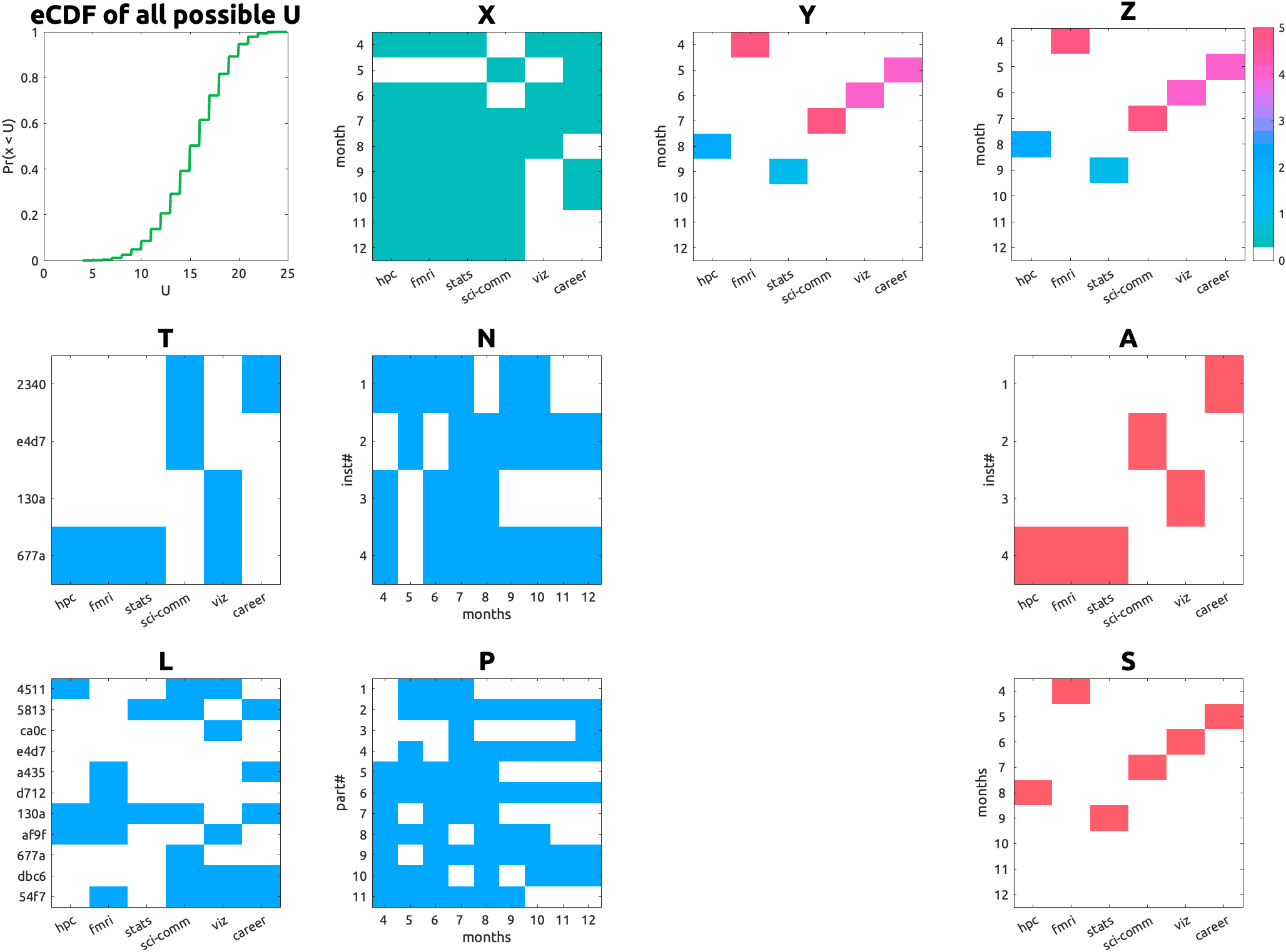Fig 1. An example solution. Names are hashed. Topic names are abbreviated.

The optimal assignment ($\mathbf{A}$; e.g., Instructor 4 does three topics) and session schedule ($\mathbf{S}$; those three topics are scheduled in July, April and September) achieves the maximal utility.

4. Joke analysis

The GOO algorithm is a joke because it is an unnecessarily complicated solution to a simple problem. It is also a joke because it is more inefficient than an exhaustive search. However, it is not a joke when the random search actually finds the optimal solution much faster than the exhaustive search. This depends on the dimensions of the problem and the arbitrary number of iterations chosen for the random search.

We can pin-point where it stops being a joke: when the number of iterations is less than the total number of possible combinations, and the random search finds a solution that is close to the optimal solution. We can do this by simply estimating bootstrapped mean utility of random solutions with different numbers of iterations, and compare it with the optimal solution.

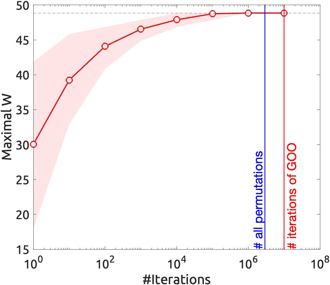Fig 2. Joke analysis.

So, from the analysis, it’s clear that the GOO iteration (10^7) is well above the Joke Horizon (i.e., the number of possible combinations). But for about 10^5 iterations, it is already actually efficient (with the GOO optimum in its 95% confidence interval) random search (killing the joke 🤓).